Fake Job Classifier

Table of contents

Concepts: Naive Bayes, SGD
Dataset
Classifier
Challenges Faced
Solutions
Experiments
Visualizations
Personal Contribution
Source Code
References

I built a classifier that identifies if the job posting is fraudulent or not with an accuracy of 84% (actual F score below in the article). There were various challenges that I faced when building this classifier and I would describe those in this article alongside the concepts that helped me overcome the challenges.

Concepts :

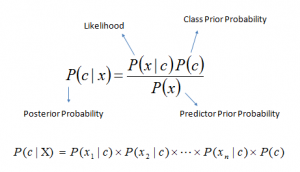
Naïve Bayes : Naïve Bayes has its foundation in the Bayes theorem. In simple words, bayes theorem helps determine the probability of an event occurring given that an event has already occurred.

Naïve in Naïve bayes is the assumption that the features(B or features in our case would be words in a sentence and A is the class of the news) are not correlated and that the presence of one would not affect the probability of that event occurring(classifying a class).

Stochastic Gradient Descent (SGD): In simple words “Stochastic gradient descent is a method to find the optimal parameter configuration for a machine learning algorithm”^[3]

SGD is actually an optimization technique for gradient descent. I have used a SGDclassifier which is not a classifier but rather its a linear classifier which is optimized using SGD. To understand SGD it is essential to understand what gradient descent means. Gradient Descent is a popular optimization technique in Machine Learning and Deep Learning, and it can be used with most, if not all, of the learning algorithms^[4]. A gradient is the slope of a function. It measures the degree of change of a variable in response to the changes of another variable.

In real life, when we implement gradient descent we come across a term called as “batch” which denotes the total number of samples from a data set that is used for calculating the gradient for each iteration. For a typical gradient descent optimization, a batch is taken to be of very large size, sometimes the whole dataset. Although taking the large sized batch helps in reaching the local minima in a less noisy and less random manner, the problem arises when the dataset gets really big like a million samples. When that happens, the batch size would make it computationally very expensive. This is where the “Stochastic” in the SGD comes into picture. Stochastic comes from the approach of “randomly” selecting a sample. The stochastic approach alongside the sample size of a single sample(i.e. batch size of one, to perform for each iteration) helps optimize the algorithm at the cost of reaching the local minima in a noisy and random manner but this doesn’t really matter as long as the local minima is reached^[4]. The image below represents the two different approaches.

For more detailed understanding you can refer to this article

Gradient Descent(smooth) vs Stochastic Gradient Descent(Noisy)^[2]

Dataset:

This dataset contains about 18K job descriptions out of which about 800 are fake. The data consists of both textual information and meta-information about the jobs.

Class representation : [0 – Genuine 1 – Fake Job]

Classifier :

I built the classifier in two ways, one using Naïve Bayes and other using SGD.
Reason for building it in two ways is I wanted to experiment with building a Naïve Bayes classifier from scratch but after seeing the result I decided to go with another approach. Both of the approaches are mentioned below.

Naïve Bayes Classifier: If you feel lost in the below explanation, you can find a more detailed explanation here(my previous article). Also you can find the exact code in the source code section below.

The first step is the data preprocessing (removing NaN’s, splitting the data into train, develop/validate, test and other such data specific processing like stemming) the next step is to build a word frequency matrix/data frame and the probability matrix/data frame which are required in order to compute the conditional probabilities and make the prediction based on that.

Script to build the word frequency matrix/ data frame

Word frequency data frame – words are reduced to their stems

Follow the same procedure as the one used to build the word frequency data frame for building the probability matrix that holds the probabilities of the words given they belong to a class.

Once we have the two above mentioned matrices we calculate the posterior probability of a class given the word combination(i.e. the sentence). The above calculations have been made after smoothing in order to avoid the zero probability problem for unseen words by the classifier.

Conditional Probability , Credits – Analytics Vidya^[5]

Upon performing the predictions on the test dataset I witnessed something unusual

F score matrix understanding – Fraud vs Genuine Job Posting

True positive is actually positive(Fraudulent) and predicted positive(Fraudulent), True negative is actually negative(Genuine) and predicted negative(Genuine). Based on the classifier prediction – we have 4 counts of job posting that were predicted genuine but were actually fraudulent while the rest 96 counts of the 100 were predicted genuine and were actually genuine.

This looks great! but in truth this is due to the fact that the data was highly imbalanced towards the genuine job postings.

It is pretty evident that the difference in the ratio of the classes. Alright what now? well, there are various ways to tackle this situation. For our case I would be be switching things up a bit. I would now be using another algorithm called SGD alongside resampling(specifically under sampling) – among the various combinations available I chose this combination since it worked well for me.

SGD Classifier: We start by performing the required pre processing of the text which includes replacing various special characters and other special character combinations such as http and also split the data for training and testing. After that I tokenized the sentences

and under sample the data so that both classes are equally represented.

Then we fit the model to get the predictions.

This time unlike the last time we would be looking at a better evaluation matrix than just the accuracy.

Precision (also called positive predictive value) is the fraction of relevant instances among the retrieved instances, while recall (also known as sensitivity) is the fraction of relevant instances that were retrieved. Both precision and recall are therefore based on relevance^[14].

Model Predicts a fraudulent job posting as fake correctly

Model Predicts a genuine job posting as genuine correctly

The output array([1]) represents that the prediction says its a fraudulent job posting while the array([0]) indicates that it is a genuine job posting.

Challenges Faced:

Imbalanced Dataset: The major challenge I faced was the imbalanced dataset. Having an imbalanced data set affects the accuracy results significantly as mentioned in detail earlier above in the article.

Evaluation Score : Just relying on the accuracy alone can lead to result interpretations that are false

Kaggle limitations : Often times the notebook would crash because the notebook allocated more memory than available which lead to restarts of the notebook and this is painful because a larger dataset takes a lot of time to process and every time notebook restarts one has to wait all over again for that time consuming process to be run before you could anything further with your work.

Solutions:

Imbalanced Dataset: By means of using resampling, specifically I used under sampling. Undersampling techniques remove examples from the training dataset that belong to the majority class in order to better balance the class distribution, such as reducing the skew from a 1:100 to a 1:10, 1:2, or even a 1:1 class distribution. This is different from oversampling that involves adding examples to the minority class in an effort to reduce the skew in the class distribution^[6]

Evaluation Score : For imbalanced data sets, a better evaluation matrix/scores is a F measures^[15]

Kaggle limitations : Solved this by reducing the data set size for specific processes that lead to notebook failures.

Experiments

I experimented a little with the Naïve Bayes classifier that I made from scratch and it gave out a pretty good result of 90+ accuracy but this was due to the data imbalance. Upon visualizing the data I realized that the Naïve Bayes I built would not work that well since the words are very similar to each other for both classes (Fraud vs Genuine)which would mean that it would be difficult for the classifier to classify such close documents given the imbalance of the classes.

Fraudulent vs Genuine Job Post – Top 10 influential words

Visualizations:

Scatter plot of the TDFIDF Vector to visualize the distribution of the class wise data- the vectors represent the job postings from both the classes. Learn more about TFIDF vectorization here.

Fraud vs Genuine TFIDF vector scatter plot

Personal Contribution

Building the Naïve Bayes Classifier from Scratch.
Writing this article
Video on the classifier : https://www.youtube.com/watch?v=5leaVZxb-5E
Building visualizations : top 10 words & scatterplots
Experimenting with Naïve Bayes and Overcoming the challenges
Building SGD with reference – applying preprocessing and building visualizations